Residuals are not an insect but they still bug me

Today, I commented to one of my daughters that I was examining residuals. She asked if that was a kind of insect, like a termite. I told her no, but they still were bugging me.

To a statistician, all of the variance in the world is divided into two groups, variance you can explain and variance you can’t, called error variance.

Residuals are the error in your prediction. In a nutshell, if your actual score on say, depression, is 25 points above average and, based on stressful events in your life I predict it to be 20 points above average, then the residual (error) is 5.

In a second nutshell (or the first one, if the nutshell is really large), logistic regression is preferred to linear regression when you have a categorical dependent variable. No, it is NOT okay to just pretend your dependent is continuous. No, you are not the first person to have asked that.

In your first statistics course (or your second, if you went to a school where you took your time),  you no doubt learned about assumptions of linear regression models, that is:
(i) linearity of the relationship between dependent and independent variables
(ii) independence of the errors (no serial correlation)
(iii) homoscedasticity (constant variance) of the errors across predictions (or versus any independent variable)
(iv) normality of the error distribution.

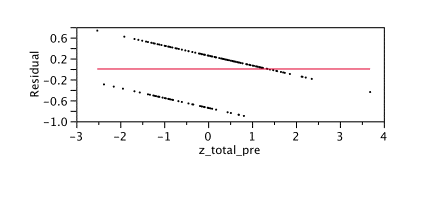
Below you can see where I plotted the residuals against a predictor (pretest score) for a dichotomous variable, passed course, coded as yes or no.

If you have an unbiased predictor, you should be equally likely to predict too high or too low. The mean of your error should be zero. It is, in fact, really close to zero here. I computed it and the mean of the error is -.0004 . It should also be zero at all points. No one is going to be too happy if you say that your predictor isn’t very good for A students. However, it seems that is exactly what’s happening. In fact, past about 1.5 standard deviations above the mean, ALL of our students have been under-predicted.

For a contrast, here is what the residual times predictor plot looks like for a continuous, numeric dependent variable, post-test score.

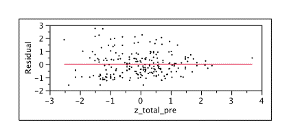Let’s go back and forth between these two and be bothered for a while. As you can see, our residuals for the continuous prediction are above and below the mean. Also, you’d think if you have a good prediction, the average error should be zero – because the too- high and too low predictions cancel out. My prediction of a continuous variable did better, with a mean of .0000000000000001 , which is closer to zero than -.0004 but, seriously, both are pretty close to zero.

Your errors should center around zero, with small errors more common than large ones. This doesn’t happen at all with the binary dependent variable. In fact, most of your errors are far above or far below mean of zero.

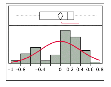
That whole constant variance across the predictors – homoscedasticity thing? The distribution of errors being normal? Yeah, not happening here. Let’s say I graph the errors. There should be  a normal distribution. Below is the graph of the distribution of errors for a binary dependent variable (predicting if the person passed or failed). A normal curve is fit over it and you can see that the fit is not that great.

Now let’s take a look at the residuals for a continuous predictor – score on the final test.

Below you see the distribution for residuals predicting the post-test score on an exam from the pretest score, that appears to be closer to a nice, normally distributed dependent variable.

The diamond indicates the mean and the median id that straight line. You can see comparing the two graphs that the median is much closer to the mean for the continuous example. I have to admit though, that there are a few more extreme outliers for the continuous dependent variable.

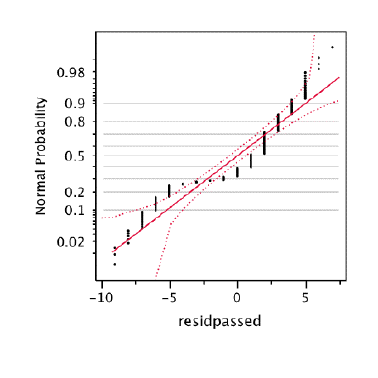
Finally, if you look at the diagnostic plots of two analyses, one with a continuous measure in logistic regression you see this normal probability plot. It should look like a straight line. When we take a look at the plot, it does look pretty much like a straight line, except for at the extremes. We have more extremely low scores and more extremely high scores than should be perceived in a normal distribution.

Pay attention! This has the continuous dependent variable first.

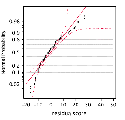When we look at the plot of the residuals for predicting the binary variable (passed versus failed) we can see that it departs from a straight line at just about every point.

So, here is what was bugging me. Normally, we tell students that they cannot use linear regression with a binary dependent variable because it violates the assumptions of regression. We show them some equations, which they believe will have very little to do with their lives after graduate school and forget immediately after the mid-term exam.

Even though it does not require the statistician secret decoder ring, I am wondering if  we might have more success with some pictures that are worth a thousand words, saying,

“Hey, when you have a variable that is 0 or 1, it is not continuous, and the results are going to be somewhat different than if you really had a linear relationship. The errors that you get should look like B but it actually looks like A. It is not profoundly different, but it is different and so you should really use the correct method.”