To specialize or not to specialize, in 140 characters or less
AN ACTUAL CONVERSATION THIS WEEK …
“This paper is not going to be as much an academic treatise as most of the ones I write, but I am hoping it will be more interesting. I was wondering about the fact that some well-respected people say the secret to career success is to be the foremost specialist in some obscure application or language. That doesn’t fit with my experience at all, though. So, instead of citing some articles I pretty much just sent a shout-out on Twitter, got responses from smart people and quoted them.”
“You mean you crowd-sourced it?”
“Gee, it sounds SO much more professional and scientific when you put it that way!”
Often there is a distinction made between programmers – who write code – and analysts, managers or other categories who use the results of that coding. Some would say that the secret to career success is to specialize. There is something about this view that bothers me, so I went to Twitter, quickly replacing Google and Wikipedia in my life as the source of all knowledge and asked fellow twitterers their opinions.
Dr. Peter Flom, a statistician replied,
I am not a programmer, but as data analyst/statistician, I think you can be successful either way
In my experience, there are a good number of people who have made a successful decades-long career as the maven of PROC REPORT or SAS/AF or some other specific niche that was of critical importance to some division of their organization.
Jon Peltier, an Excel programmer answered,
Depends on how much in demand your specialty is.
Evan Stubbs, of SAS Institute in Australia put it best when he succinctly summed up what bothers me about the specialization paradigm.
Fly high, fall far; pay’s good for specializing until you go the way of the buggy whip. Generalists fit anywhere, learn faster
Let’s be generalists then, and apply what we know about SAS to answer some questions using statistical procedures. In the first part of SAS Essentials, I said that one distinction between a novice and an intermediate programmer is being able to make design choices because he or she knows more than one way to achieve a task. A second distinction is being able to put together the things you know
We’re going to try to put together some of the procedures you may know to understand a bit more about an incomprehensible subject – hate crimes. These are crimes that are motivated by bias against the victim’s race, religion, sexual orientation or disability status. We’ve already seen in a prior example the most common categories. How often does this happen and what do hate crimes look like? I want to start with the victims and offenders so I use PROC UNIVARIATE. The code below will give some initial statistics for both the number of victims and the number of offenders ;
ODS GRAPHICS ON ;

Proc univariate data = in.hatecrime plots ;

Var tnumvtms tnumoff ;

Where hc_flag = 1 ;
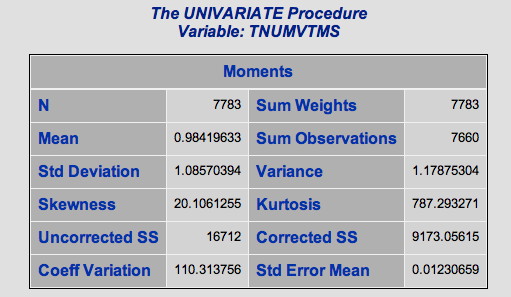
The first set of results is very interesting. This tells you that there were 7,783 hate crimes in the database in 2008 and the average had slightly less than one victim. Of course, this is very curious so let’s explore it further.
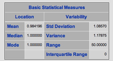
In the table below, both the median (the score that half of the population falls above and half fall below) and mode (the most common score) are one. So, in general a hate crime seems to be perpetrated against an individual. In a normal distribution, the mean = the median = the mode. This would seem to meet that criteria with the mean for number of victims = .98, median = 1 and mode = 1. Yet, according to the statistics in the table above, the distribution is very far from normal. You can see this by looking at the skewness and kurtosis statistics, which are enormous.[1] A kurtosis value for a normal distribution is 0. Ours is 787. Skewness measures how symmetric (or not) the curve is and kurtosis measures how flat or peaked it is (in contrast to the “bell” shape we would expect in a normal curve.
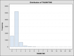
The standard deviation is about one, again, suggesting that most crimes are committed against a solitary victim with not a lot of variation from the mean. To gain a little more understanding, let’s take a look at the frequency distribution produced by PROC UNIVARIATE when we used the ODS GRAPHICS ON statement.
What this picture shows is that hate crimes are overwhelmingly likely to have only one victim. The next most common number is zero, which is weird, but we’ll get back to that in a minute.
In this case, the results shown in the next table, the t-test that the population mean is zero isn’t of much interest to us. If I’d included this table (which I didn’t because it was irrelevant and hence boring), we could see, unsurprisingly, that it is hugely significant. No real information here – the average number of victims of a hate crime in the population is not zero (duh). There are times when this statistic would be of interest. This isn’t one of those times.
The next table is quite interesting, though. It gives the responses in quantiles, from 0% to 100%. The minimum number of victims, and, in fact, up to the tenth percentile, is zero.
When I look at the results for the number of offenders, I find a similar pattern, where 10% of the records show zero offenders.
Something is definitely strange here, how can you have crimes with no victims and no offenders, and, if so, how do you know they are hate crimes? To learn a little bit more about this, I do the following:
data in.check ;
attrib victim_off length = $11. ;
if hc_flag = 1 ;
if tnumvtms = 0 and tnumoff > 0 then victim_off = “No victim” ;
else if tnumvtms > 0 and tnumoff = 0 then victim_off = “No offender” ;
else if ( tnumvtms = 0 and tnumoff = 0) then victim_off = "Neither" ;
else if ( tnumvtms > 0 and tnumoff > 0) then victim_off = "Both" ;
proc freq data = in.check ;
tables offcod1 * victim_off ;
where victim_off ne "Both" ;
The above code creates a dataset that only includes hate crimes (hc_flag = 1). It also creates a variable victim_off , that has four categories, no victim, no offender, neither victim nor offender or both a number of victims and offenders given. The FREQ procedure shown creates a cross-tabulation of the offense code by the victim_off category.
… and it becomes somewhat clear to me by reviewing the offense codes in the resulting table which I did not show because I am by now tired of showing tables in this post.
About two-thirds of the cases with no victim and/ or no offender are destruction or vandalism. So, if someone trashes a church or synagogue and leaves behind spray-painted racist or anti-semitic comments, that would be considered a hate crime and you would have an identifiable group that the bias was motivated against, but there wouldn’t necessarily be an identified victim.
The next step simply requires going back to the documentation. It turns out that if the offender is unknown, a zero is entered in this field.
This is just a tiny, beginning part of an analysis. Why even bother?
Let’s say you are a brand new programmer that maybe just finished your first SAS class that your company sent you to, so some code with a few IF statements, a PROC FREQ is a reasonable expectation from you. You proudly hand over your charts and tables and someone says,
“How the hell can you have zero victims and zero offenders for a hate crime?”
You can kind of shrink back into yourself and say,
“I don’t know.”
or, You can very defensively and somewhat aggressively state,
“How should I know, that’s not my job. I’m just the programmer.”
Or you could say …
“Well, it’s like this …”
Even if you’re a brand-new baby programmer that is just learning to cobble together a data step and a proc freq, I can tell you that in most organizations one of those three answers is going to get you more respect than the others.
[1] The formula for kurtosis sometimes subtracts 3 (which makes the value for a normal distribution equal to 0), and sometimes doesn’t. SAS software uses the formula that subtracts 3.


One Comment