Travels through Open Data Land, with old people, flashlights & cigars

(Yes, that title does sound like a lot of the spam comments I get. )

Last year, at the Gov. 2.0 conference in Santa Monica, Jean Holm, from NASA spoke about some of the opportunities for open data. I left with mixed feelings. On the one hand, the best examples she gave were, I thought, of  “semi-open” data, that is, a term I just made up for having more openness of data within an organization.  In one example, there would be a database of the capabilities of researchers within NASA, so if I was a NASA electrical engineer and I had an idea for designing a better electrical system for a lunar module, I could find out who had related expertise in hardware design, reliability testing, etc. That is a great idea, but it also makes me wonder to what extent open data within an organization would be put to use. It depends a lot on the organization.  Many large institutions – whether corporate, government, non-profit or educational – are not very excited about people going around the usual chain of command or departmental structure, no matter how many times they chant, “Think outside the box!”

Many times, both on this blog and elsewhere, I’ve questioned the probability of useful discoveries coming from open data unless the individuals doing the analysis have some knowledge of statistics, programming and the structure of the data actually being used .  If we have ten thousand each people doing 100 analyses, how do we decide which half of the 100,000 statistically significant results is important and which are in the group of 50,000 statistically significant results we would expect to occur by chance with 1,000,000 analyses?

Ten thousand people doing 100 analyses = 1,000,000 results.  One of those will have a p-value of .0000001 just by chance. A one in a million coincidence happens one time out of a million, right? So, let’s say we get three of those p < .0000001 events. How do we know which ones matter?

 

She said, sure you can have people correlating everything and come up with nonsensical relationships like between number of flashlights sold and solar flare activity. Presumably, somewhere “out there” are scientists or consumers of data or someone who will be able to identify the real findings from the flashlight sales- solar flares relationships. Having read a lot of academic journal articles that appear to have been both written and edited by people who were either not paying attention, inebriated or both, I am not so optimistic.

So, I decided to do an experiment and see just how far I could get with some samples of open data. The first data set I chose was from the Kaiser-Permanente study of the oldest old. This is actually two data sets.

One of the reasons I chose these data are that they come with pretty comprehensive documentation. For example, after reading through several hundred pages, I knew that the first data set was the master file and the second was a hospitalization file. In my experiment to see if I could find anything useful in here at all (other than what had already been published), I decided to use just the master file.

A second reason for selecting the oldest old study is that there are some published statistics I can verify my results against to see whether I have the data read in and coded correctly from the beginning. For example, the number of deaths I had in the first cohort (1,565) and second cohort (1,751) matched their figures exactly.

I did not start out with any preconceived notions other than the general public, assumptions like the older people were at the beginning of the study, the more likely they were to die before it was over.  While I’ve worked on some health statistics studies in the past, I am not a physician. This is one reason I used the master file, instead of the hospitalization one. I know what acute myocardial infarction is but I could not really generate much in the way of hypotheses about it nor the accuracy of diagnosis.  On the other hand, dead or not dead is pretty objectively measured.

I started with cigar smoking because I have a friend who turned 65 last month. His annual physical went like this:

Doctor: Do you still smoke cigars?

Jim: Yep.

Doctor: Do you still drink 8 or 9 beers every night?

Jim: Yep.

Doctor: Are you going to quit?

Jim: Nope.

Doctor: Well, see you next year.

You know how old people always tell you that it doesn’t matter if they quit now, because they’re too old to die young anyway? I got to wondering if that was true, if people who were smoking and still alive at age 65 would be any more likely to die. (We’ll save the 8 or 9 beers thing for later.)

My first analysis was to look at the data by gender because I suspected that men were more likely to smoke cigars and I knew that women have  a longer life expectancy. When I did a table analysis by gender and cigar smoking using SAS Enterprise Guide, I found that only one of the 288 cigar smokers in the sample was female. So, it was clear to me if I was looking at the impact of cigar smoking on mortality I should probably only look at men.

The average age at death for men who smoked cigars (N=175) was 84.2 years, compared to 84.2 years for men who did not smoke cigars (N=1,147). Since there was some rounding here, p does not equal exactly 1.0 but rather p > .90.  So, it does not seem that quitting cigar smoking would improve your life expectancy given you have already made it to age 65.

However, that is only people who died. Perhaps not smoking will increase your probability of survival? Let’s just take a simple chi-square analysis comparing people who smoked cigars to those who did not and seeing what is the probability they died over the nine years they were followed.

Of the cigar smokers, 13.2% died during the nine years participants were followed, compared to 13.1% of men who did not smoke cigars (chi-square = .07, p > .78).

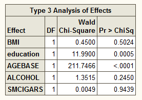
Still, I am not convinced. Maybe cigar smokers were older, or less likely to be overweight or drink (well, I doubt that one).  Anyway, being the good little statistician, I ran a logistic regression with death as the dependent variable and BMI, education, age at the beginning of the study (baseline), whether or not the subject had ever drank alcohol and whether or not he smoked cigars as the predictors.

As you can see, the only two significant factors were age (older people were more likely to die in the next nine years – not surprisingly since the study began with people 65 and over) and your education. I’m guessing education is a proxy for social class.

So, it looks as if Jim is okay to keep smoking his cigars, given he has made it this far. I’m still not convinced about the 8 or 9 beers, though. That’s my next analysis.